
Visualisierung der Kohlendioxidmessung Teil 7
Die Konzentration ist im Mai auf der Nordhemisphäre am höchsten, da das im Frühling stattfindende Ergrünen zu dieser Zeit beginnt; sie erreicht ihr Minimum im Oktober, wenn die Photosynthese betreibende Biomasse am größten ist.
Stand: 27.04.2021
import locale
locale.setlocale(locale.LC_ALL, 'de_DE')

import numpy as np
import matplotlib.pyplot as plt
import matplotlib.style as style
style.use('fivethirtyeight')
from calendar import month_abbr


df_vis = pd.read_csv('daten/wasserkuppe.csv')
df_vis.index = pd.to_datetime(df_vis.Datum)

df_vis
| Datum | Temperatur | Luftdruck | Kohlendioxid | |
|---|---|---|---|---|
| Datum | ||||
| 2000-05-07 01:00:00 | 05-07-00 01:00 | 9.7 | NaN | NaN |
| 2000-05-07 02:00:00 | 05-07-00 02:00 | 9.8 | NaN | NaN |
| 2000-05-07 03:00:00 | 05-07-00 03:00 | 9.7 | NaN | NaN |
| 2000-05-07 04:00:00 | 05-07-00 04:00 | 9.4 | NaN | NaN |
| 2000-05-07 05:00:00 | 05-07-00 05:00 | 8.8 | NaN | NaN |
| ... | ... | ... | ... | ... |
| 2020-04-06 20:00:00 | 04-06-20 20:00 | 8.8 | 994.0 | 735.0 |
| 2020-04-06 21:00:00 | 04-06-20 21:00 | 8.8 | 995.0 | 737.0 |
| 2020-04-06 22:00:00 | 04-06-20 22:00 | 8.8 | 995.0 | 739.0 |
| 2020-04-06 23:00:00 | 04-06-20 23:00 | 7.6 | 995.0 | 740.0 |
| 2020-05-06 00:00:00 | 05-06-20 00:00 | 6.5 | 995.0 | 737.0 |
174600 rows × 4 columns
df_vis = df_vis.resample('M').mean()
df_vis
| Temperatur | Luftdruck | Kohlendioxid | |
|---|---|---|---|
| Datum | |||
| 2000-01-31 | 9.597414 | NaN | NaN |
| 2000-02-29 | 6.987156 | NaN | NaN |
| 2000-03-31 | 5.985321 | NaN | NaN |
| 2000-04-30 | 5.805000 | NaN | NaN |
| 2000-05-31 | 6.943972 | NaN | NaN |
| ... | ... | ... | ... |
| 2020-08-31 | 5.670833 | 1020.233333 | 751.100000 |
| 2020-09-30 | 7.174167 | 1014.941667 | 745.800000 |
| 2020-10-31 | 5.693333 | 1009.225000 | 741.425000 |
| 2020-11-30 | 2.715833 | 1012.291667 | 745.200000 |
| 2020-12-31 | 2.384167 | 1013.800000 | 746.466667 |
252 rows × 3 columns
t = df_vis['Temperatur']
p = df_vis['Luftdruck']
mol = 44.01
mg2 = df_vis['Kohlendioxid']

df_vis['ppm'] = 10*mg2/mol*((8.31447*(t+273.15))/p)

df_vis
| Temperatur | Luftdruck | Kohlendioxid | ppm | |
|---|---|---|---|---|
| Datum | ||||
| 2000-01-31 | 9.597414 | NaN | NaN | NaN |
| 2000-02-29 | 6.987156 | NaN | NaN | NaN |
| 2000-03-31 | 5.985321 | NaN | NaN | NaN |
| 2000-04-30 | 5.805000 | NaN | NaN | NaN |
| 2000-05-31 | 6.943972 | NaN | NaN | NaN |
| ... | ... | ... | ... | ... |
| 2020-08-31 | 5.670833 | 1020.233333 | 751.100000 | 387.798992 |
| 2020-09-30 | 7.174167 | 1014.941667 | 745.800000 | 389.157172 |
| 2020-10-31 | 5.693333 | 1009.225000 | 741.425000 | 387.010451 |
| 2020-11-30 | 2.715833 | 1012.291667 | 745.200000 | 383.661572 |
| 2020-12-31 | 2.384167 | 1013.800000 | 746.466667 | 383.280561 |
252 rows × 4 columns
df_vis = df_vis.drop(columns=['Temperatur','Luftdruck','Kohlendioxid'])
df_vis
| ppm | |
|---|---|
| Datum | |
| 2000-01-31 | NaN |
| 2000-02-29 | NaN |
| 2000-03-31 | NaN |
| 2000-04-30 | NaN |
| 2000-05-31 | NaN |
| ... | ... |
| 2020-08-31 | 387.798992 |
| 2020-09-30 | 389.157172 |
| 2020-10-31 | 387.010451 |
| 2020-11-30 | 383.661572 |
| 2020-12-31 | 383.280561 |
252 rows × 1 columns
Folgender Code war bei der Erstellung hilfreich [^1]
co2_data = df_vis['2011':'2019']
n_years = co2_data.index.year.max() - co2_data.index.year.min()
z = np.ones((n_years +1 , 12)) * np.min(co2_data.ppm)
for d, y in co2_data.groupby([co2_data.index.year, co2_data.index.month]):
  z[co2_data.index.year.max() - d[0], d[1] - 1] = y.mean()[0]

plt.figure(figsize=(10, 14))
plt.pcolor(np.flipud(z), cmap='hot_r')
plt.yticks(np.arange(0, n_years+1)+.5,
           range(co2_data.index.year.min(), co2_data.index.year.max()+1));
plt.xticks(np.arange(13)-.5, month_abbr)
plt.xlim((0, 12))
plt.colorbar().set_label('Kohlendioxidmessung in mg/m³ der Messstation Wasserkuppe ')
plt.show()
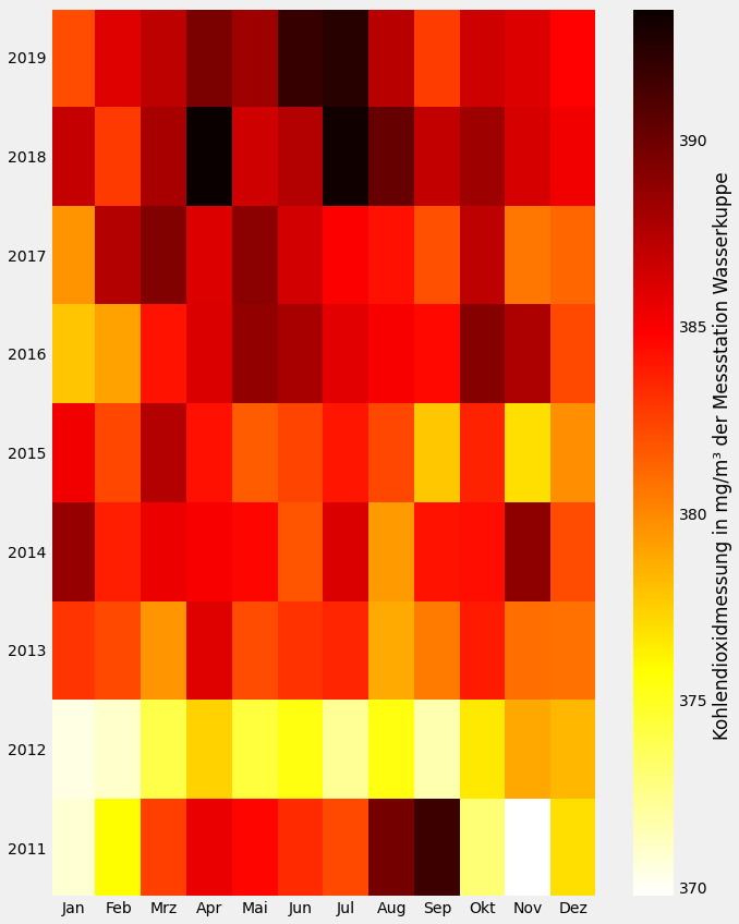
In der Abbildung sind die Kohlendioxidwerte für November 2011 am geringsten und im April 2018 am höchsten. Der Einfluss der Nordhemisphäre dominiert den jährlichen Zyklus der Schwankung der Kohlenstoffdioxidkonzentration, denn dort befinden sich weit größere Landflächen und somit eine größere Biomasse als auf der Südhemisphäre. Die Konzentration ist im Mai auf der Nordhemisphäre am höchsten, da das im Frühling stattfindende Ergrünen zu dieser Zeit beginnt; sie erreicht ihr Minimum im Oktober, wenn die Photosynthese betreibende Biomasse am größten ist.1
Minimale und maximale Werte
Anschließend werden die maximalen und minimalen Werte aufgelistet.
t = pd.to_datetime('11-11-30')
t

df_wasserkuppe_01_02_2002_12_0 = df_vis[(df_vis.index == '2011-11-30')]
df_wasserkuppe_01_02_2002_12_0
| ppm | |
|---|---|
| Datum | |
| 2011-11-30 | 369.717896 |
df_wasserkuppe_01_02_2002_12_0 = df_vis[(df_vis.index == '2018-07-31')]
df_wasserkuppe_01_02_2002_12_0
| ppm | |
|---|---|
| Datum | |
| 2018-07-31 | 393.254659 |
df_vis['ppm'].argmax()
219
df_vis.iloc[[df_vis['ppm'].argmax()]]
| ppm | |
|---|---|
| Datum | |
| 2018-04-30 | 393.527525 |
df_vis.iloc[[df_vis['ppm'].argmin()]]
| ppm | |
|---|---|
| Datum | |
| 2011-11-30 | 369.717896 |
Quellenangaben: [^1]: Vettigli, G. (2019, 22. April). Visualizing Atmospheric Carbon Dioxide. Dzone.Com. https://dzone.com/articles/visualizing-atmospheric-carbon-dioxide
U.K. (2016, 21. Januar). Florierende Vegetation verstärkt Kohlendioxid-Schwankungen. Max-Planck-Gesellschaft. https://www.mpg.de/9862783/co2-schwankung-vegetation-erderwaermung ↩